| Week 8 | |
|---|---|
| Course | Arch 2042 |
| Date | 2012/04/20 |
| Learning Objectives | We will start our treatment of meshes by providing specific examples of situations in which structured meshes play a role. In particular, we will revisit transformations and see how the concepts of basis, coordinates and coordinate systems underly most strategies for aggregation and tiling. |
| Agenda |
|
| Uses Tool(s) | |
Structured Meshes
In class we worked through this example of how to create a polygon mesh of a parametric surface, where the mesh directly results from the isocurves. Add the function to the file DrawParametricSurface.py to generate meshes of surfaces.
def DrawMeshParametricSurface(parametric_equation):
    "Generates and draws a mesh for a surface based on a parametric description."
    # Currently only for a rectangular domain - get the minimum and maximum
   #  parameters for this domain
    u0 = rs.GetReal("Minimum u value", 0.0)
    if( u0==None ): return

    u1 = rs.GetReal("Maximum u value", 2*math.pi)
    if( u1==None ): return

    v0 = rs.GetReal("Minimum v value", 0.0)
    if( v0==None ): return

    # Get the maximum parameter
    v1 = rs.GetReal("Maximum v value", 1.0)
    if( v1==None ): return

    # Get the number of sampling points to interpolate through
    count = rs.GetInteger("Number of points in both u and v directions", 50, 2)

    #Create vertices of mesh
    vSurface = []
    step_u = (u1-u0)/count
    step_v = (v1-v0)/count
    for i in range(count+1):
        u = u0 + i*step_u
        for j in range(count+1):
            v = v0 + j*step_v
            point = parametric_equation(u,v)
            vSurface.append( point )

    #Create faces of mesh
    fSurface = []
    for i in range(count):
	for j in range(count):
	    curIndex = i*(count+1)+j
	    fSurface.append( [curIndex, curIndex+1, curIndex+count+2, curIndex+count+1] )

    rs.AddMesh(vSurface, fSurface)
Aggregation and Tiling
Example: Pinwheel Tiling
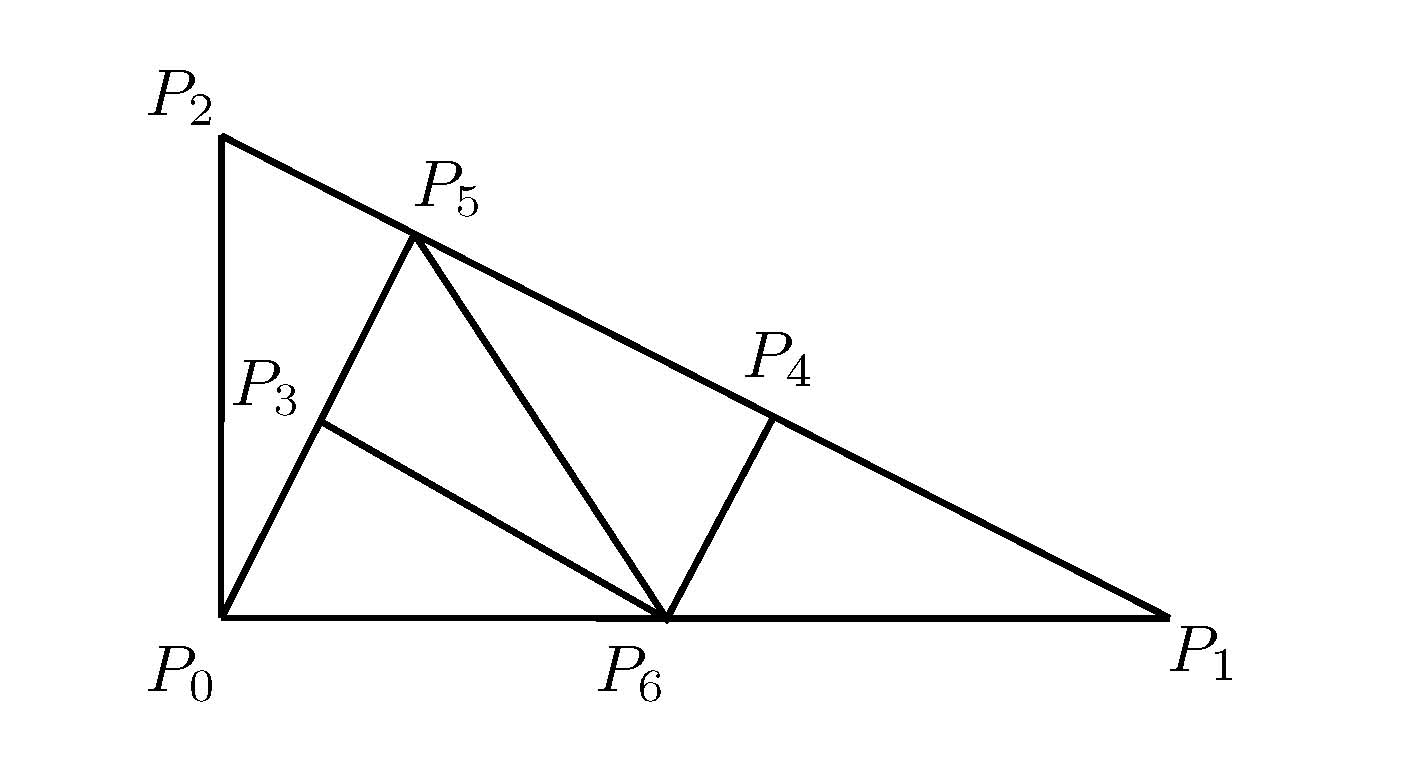
This pinwheel tiling can either be seen as a "master" described by a mesh with vertices <math> = [P_0, P_1, P_2, P_3, P_4, P_5, P_6 ] </math> and faces <math> = [[3, 6, 5], [4, 5, 6], [0, 6, 3], [0, 5, 2], [1, 4, 6]] </math> or it can be seen as a tiling generated by one unit that is replicated and transformed.
In the first case, we can think of transforming the master where the relationship of the units relative to the master stays the same. In the second case, a base unit is transformed to generate the master. In either case, transformations are put to integral use to generate combinations of highly differentiated patterns.
Tiling is all about a collection of units that are being transformed and aggregated together. Let's see how the concepts of basis, coordinates and coordinate systems can be used to efficiently generate these tilings computationally.
Basis, Coordinates, Coordinate Systems
Application to Computational Tiling
For the pinwheel example, it is easy for the eye to make the necessary adjustments (of translation, rotation, flipping, scaling etc) to recognize that the same unit is in fact being transformed to generate tilings, but to a computer, these transformed units all look different. With the help of basis and coordinate systems, we will see how the following transformed versions of the base unit (drawn in red) are "seen" as the same unit.

- For the "rotated" unit, we can introduce a coordinate system that results from rotating the standard basis by the same amount as the tile. In rhinoscript, this can be done with rs.XformRotation which takes an orthonormal frame to another.
- For the "flipped" unit, we can introduce a coordinate system that results from the basis <math> \{-\vec e_1, \vec e_2 \}</math>
- For the "scaled" unit, we can introduce a coordinate system that results from the basis <math>\{0.5\vec e_1, 0.5\vec e_2 \}</math>.
In each of these coordinate systems, the coordinates of the vertices are <math>\left[\begin{array}{c}2\\0\end{array}\right]</math> and <math>\left[\begin{array}{c}0\\1\end{array}\right]</math>, and thus these tranformed units can be represented, manipulated and drawn identically.

