| Week 03 - Model Translations | |
|---|---|
| Course | Arch 100a |
| Date | 2013/09/13 |
| Learning Objectives | This class will continue to build upon the tools and methods learned in Week 02. Students will create three dimensional analytic drawings of their design that describe the spatial composition of the models as well as the overall concept. We will then cover physical modeling techniques to allow the students to develop a reciprocal relationship between the analytical diagrams and the constructed model. |
| Agenda |
|
| Uses Tool(s) | Rhinoceros for OSX , Illustrator CS5 |
Axonometric and Analytical Drawings
Last week we looked at creating orthographic drawings such as plans and sections to describe the formal geometry and overall composition of your models.
This week we will look at creating 3-dimensional analytic drawings of your design. These can be effective tools for describing the 3d composition of your models as well as your overall concept. There should be a reciprocal relationship between the analytical diagrams that you produce and the physical and tectonic representation of your model. Each one should inform the other.
One type of analytical drawing that we will look at is the axonometric drawing. An axonometric projection is a 3d orthographic projection that is inclined to each of the three principal axes of the object relative to the plane of projection. An advantage of axonometric drawings is that they represent an object in 3d without perspective and therefore are still measured drawings.
Lineweight Hierarchy
In axonometric drawings , the conventional order of lineweight hierarchy is as follows:
- Edges or boundary of the form (either edges along the outside of the object and the background as well as edges of an object protruding in space)
- Planar corners (two or more surfaces touching each other and creating an edge)
- Surfaces lines or details (no change in form)
Rendering
In 3d analytical drawings and diagrams, it is often times helpful to render or shade the object in order to emphasize its formal attributes and spatial depth. While we will look at much more advanced rendering techniques using Rhino and V-Ray later this semester, for the purposes of this exercise we will look at how to achieve a rendered effect in both Rhino and Illustrator.
<EXAMPLES>
Axonometric Drawing Workflow
- Workflow - Creating an Axonometric Drawing
- This workflow will show the steps to produce an axonometric drawing using an existing digital model. The final drawing will be composed of both linework that has been edited and cleaned-up on top of a simple Rhino rendered image of the digital model.
Rendering with Tone in Illustrator
An alternative and acceptable method to rendering your drawings in Rhino is to do so using tones and fills in Illustrator. This applies to both your orthographic as well as your axonometric and analytic drawings.
The following steps outline how to use these tools for orthographic projections in Illustrator. The same methods can be applied to axonometric projections.
You can use this digital model file for the orthographic projections: Orthographic Digital Model .
Cleaning Up Linework
Last week we looked at organizing linework onto appropriate layers after using the Make2d command. When working with fills in Illustrator, it is also very helpful to clean up your linework properly in Rhino first.
Creating Fill Layers
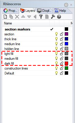
We will use the digital model to understand how we will shade the surfaces of the sheared axonometric model. To do so, right click on the view name and select Shaded. This will help us to assign proper tones. Create three new layers for the different tones. Example: light fill, medium fill & dark fill.
- New Fill Layers
Starting with the "light fill" layer, use the Polyline tool to trace over the edges that define surfaces that are in the foreground. When creating fill layers it is important to treat them like a section cut. Make sure to create a "closed curve" by ending the polyline at the exact point in which it was started. Note: The "light fill" surfaces will reflect the "light" line weight layer that was previously defined.
Continue this operation for subsequent fill layers. Some areas to fill are already defined as "closed curves." Within our specific model they are represented by many of the curvilinear holes. For these simply Copy them Inplace and assign them to their rightful "fill layer."
- Trace & Copy Fill Layers
You will notice that there are some areas that cannot be easily traced or copied. This is because they contain curvilinear curves and are represented by two or more objects. For these situations we will use the Join command. First, Copy the objects that define the area to fill away from the drawing.
Trim the objects accordingly and Join the remaining curves into a "closed curve." Finally, using the Properties Panel, assign the new closed curve to its rightful fill layer and Move it back into its proper place within the original drawing.
- Trim & Join
Now we can export our linework to Illustrator. Refer back to the Week 02 Session page for a recap of how to export from Rhino to Illustrator.
Filling the Section Cuts
You can use this file for the exported Illustrator linework: Orthographic Linework .
First import your Rhino linework into Illustrator. Since we already have our lifework organized onto layers, we can begin to use FILLS in order to describe the section cuts and the surfaces in elevation.
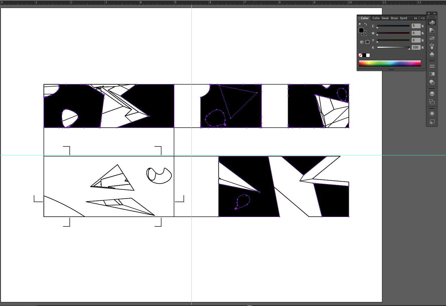
First, select all of the line work within the "dark fill" layer. This layer will represent the solid areas of our section cuts. This is easily done by clicking on the circular icon to the right of the layer within the layers panel.
After selecting, make the FILL black. FILL is the complete square icon that is next to the STROKE hollow square icon within the COLOR PANEL.
- Section Filled
Notice how the section cuts polylines that we assigned in Rhino have been filled with black. We can see that the smaller openings throughout each section have erroneously been included within the fill. Undo, or Control + z the fill command.
Now, to carry the operation out successfully, select all contents of the "dark fill layer." And open the PATHFINDER PANEL by selecting "Window > Pathfinder" from the top drop down menu.
Click on the DIVIDE button within the PATHFINDER PANEL. It is the one near the bottom left corner.
- Divide
Now the smaller section holes have been divided away from the larger section cuts. The last step before we can remove the smaller holes is to UNGROUP them. With the "dark fill" layer selected, either select "Object > Ungroup" or simply press Control + Shift + g .
Again, FILL the section layer contents with black. Now we can simply select the holes that we ungrouped and delete them.
Finally, select the "dark fill" layer contents and adjust the tonal value of the black fill within the color panel. You can do this by manually adjusting the slider for the black, or grayscale, value.
- Tonal Adjustment
Adjust the "dark fill" layer FILL to 75% black.
Filling the Elevation Surfaces
Now we will treat the elevation surfaces in the same manner as the section fill. Make the FILL values for the surfaces as follows. Also, while changing the FILL values, make sure to remove their STROKE value. This can be done by selecting the icon of a white box with a red line through it.
• Light Fill Layer - 5% black
• Medium Fill Layer - 20% black
• Dark Fill Layer - 60% black
Feel free to experiment with different tonal values.
- Filling Surfaces
Adjusting Line Weights
Now we can begin to adjust the line weights within our drawings. Open the STROKE panel by either selecting it from the right tool bar or selecting "Window > Stroke."
Select individual layers and assign them the following stroke values.
- "Section" Layer - 1pt
- "Thick" Layer - .75pt
- "Medium" Layer & "Section Markers" Layer - .5pt
- "Thin" Layer, "Hidden" Layer & "Construction" Layer - .25pt
Physical Modeling
Digital to Physical Translation
In all methods of architectural representation, it is important to communicate not just the "facts" of the design, but also the intention behind the design. This is also true for physical models, which can be used to reinforce and extend the logic behind your concept. Remember, you should be developing a synthetic process of representation, in which the techniques that informed your photomontage should then inform the manner in which you make your drawings and how you build and construct the physical model. There should be a reciprocity in your work - the model and the diagram should inform each other.
3d Physical Modeling Techniques
Laminating/Contouring
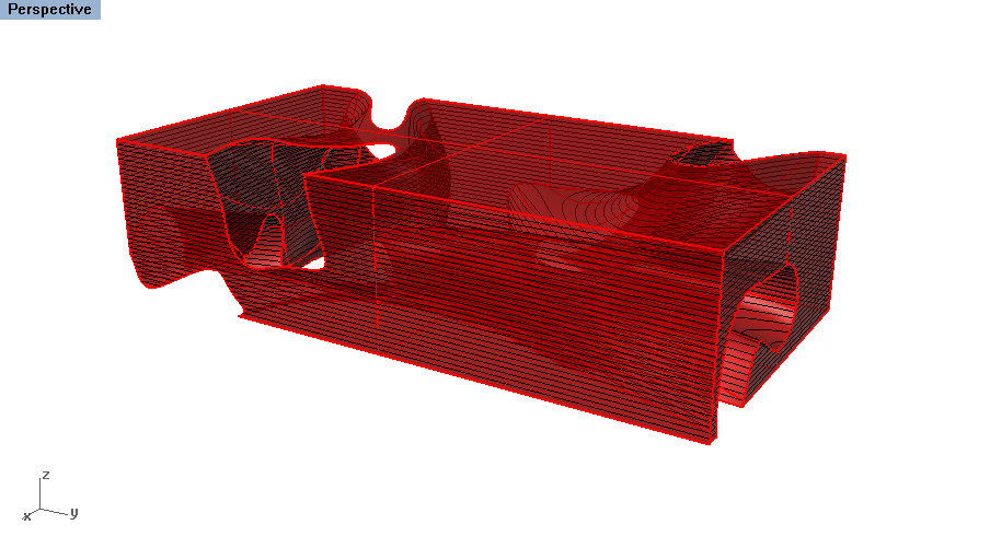
Laminating is a method of physical modeling that involves stacking pieces of material on top of each other to create a singular volume. In Rhino this is acheived by Contouring a Polysurface . It can be a helpful tool for physically modeling curved geometries.
Material
The choice of material is also important because of how the revealed edges will look. For example, if the model is made of corrugated cardboard, then the corrugation will be revealed on the outside of the model. The sides of the model will therefore look very different than the top and bottom faces of the model. The corrugation will also look different depending on how you cut the cardboard (i.e. parallel to the corrugation vs. perpendicular or diagonal).
The thickness is also important. A thin material will create a much smoother form because of the higher frequency of layers.
Unfolding
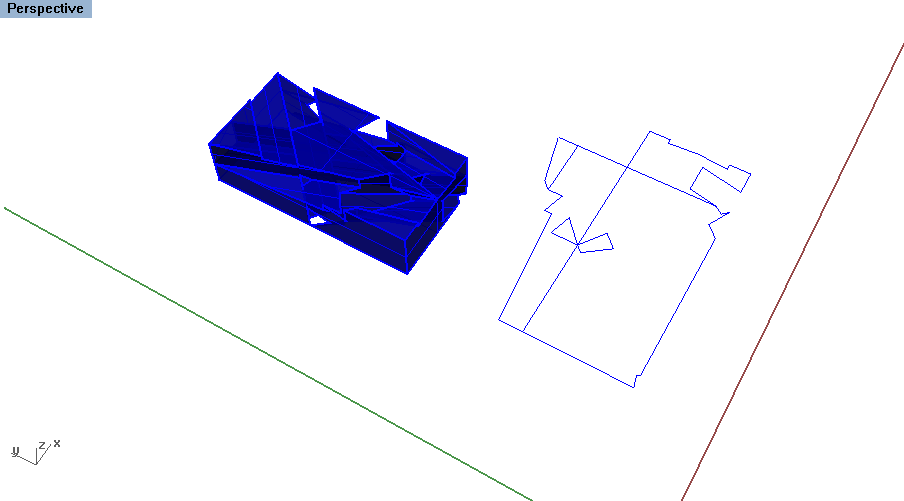
Unfolding a Polysurface enables you to flatten all of the individual surfaces of a volume onto a single plane, while still maintaining some of the connections between them. Think of it as literally unfolding a cardboard box until all sides lie flat on the ground without overlapping each other. The benefit of doing this for physical models is that the surface can then be cut out of a single piece of material and folded back into a closed polysurface.
Material
When using the UnrollSrf command, it's important to consider the thickness of the physical material you are modeling with. This technique as described above is for folding paper models, where the material thickness is essentially negligible. For thicker materials, surfaces will need to be trimmed in order to account for the thickness of the adjacent material. This is one reason why it's helpful to have the digital model scaled down to the actual size of the physical model.
Surface Modeling
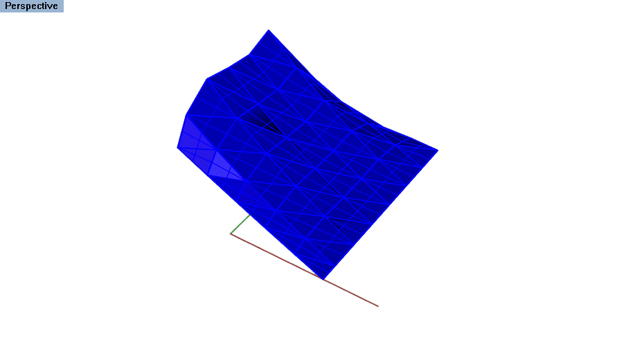
Tesselating NURBS Surfaces is a way of restructuring the geometry of complicated surfaces such that they are more easily fabricated. It is essentially involves taking a curved surface and rebuilding it with a series of small triangles. This is a good way of approximating a curved surface, though it will not be exact. However, for physical modeling purposes, this is often the best way to tackle complex, curving surfaces.
Other Methods
- 123 Make by Autodesk
- This website offers a plugin that automatically creates file templates for both laminated and waffle models. Works best for simple forms.
- Fabricating a Digital Form Using the Triangulation Method
- This workflow demonstrates the use of 123dmake to unfold, lasercut, and fabricate a mesh model. Note that to follow this workflow, you would have to convert your NURBS model into meshes.
- Waffle Method Workflow
- Written by Johanna Kanerud, Rhino file with instructions here .
Additional Resources
- Composing an Exploded Axonometric Drawing with Rhino, Photoshop & Illustrator
- This workflow explores methods of composing an exploded axonometric rendering. The working process between Rhino, Photoshop and Illustrator is emphasized; along with precision, layer organization, and composition.

